Have you heard about the benefits of the VLOOKUP function in Excel but are having trouble getting started? In this blog, I share how using a practical example and providing an example file so you can follow along!
The Setup for Our Example
In this example, we are imagining that we have a list of contacts, perhaps a registration list for a webinar or people who clicked an ad. Our objective is to distribute these contacts to our sales team for followup, but we need to make sure each salesperson only gets the contacts for companies they manage.
That's where our second spreadsheet comes in. We pulled it from our CRM system, and it includes basic information about each company, including its assigned account manager. Now we could go line by line and copy-paste the Account Manager for each company to each contact, but that's time-consuming! In reality, each spreadsheet could have hundreds or thousands of entries. Instead, let's use VLOOKUP to help.
As a preliminary step, I have opened the Contacts spreadsheet and added a New Sheet at the bottom of our workbook where I copy-pasted the entire Companies export I received from my CRM. I have created new columns that I want to fill in: Column G for Owner (where I want the Account Manager's name to appear) and Column E for Industry (where I want to see the industry name for each contact's company).
You can download the XLSX file I used for this example so you can follow along.
Step-by-Step Instructions for the VLOOKUP Function
If you would like to go through a guided ClickLearn exercise, click the link below.

Note: To advance the demo, you need to actually click where directed.
Otherwise, continue below to see each step in the process.
- Click on the cell G2 under the Owner column.
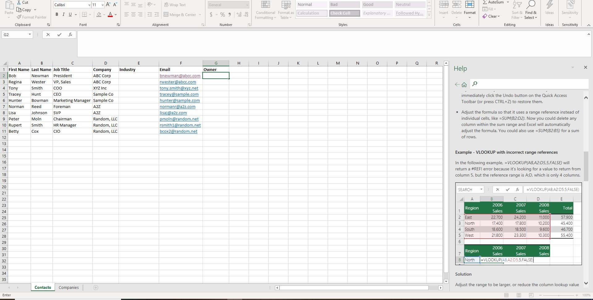
- Enter the text =vlookup(

- Click on the cell D2 with the value ABC Corp. This adds the reference to column D, where we have the company name for each contact, to our formula. We will use this value to match with a company record.
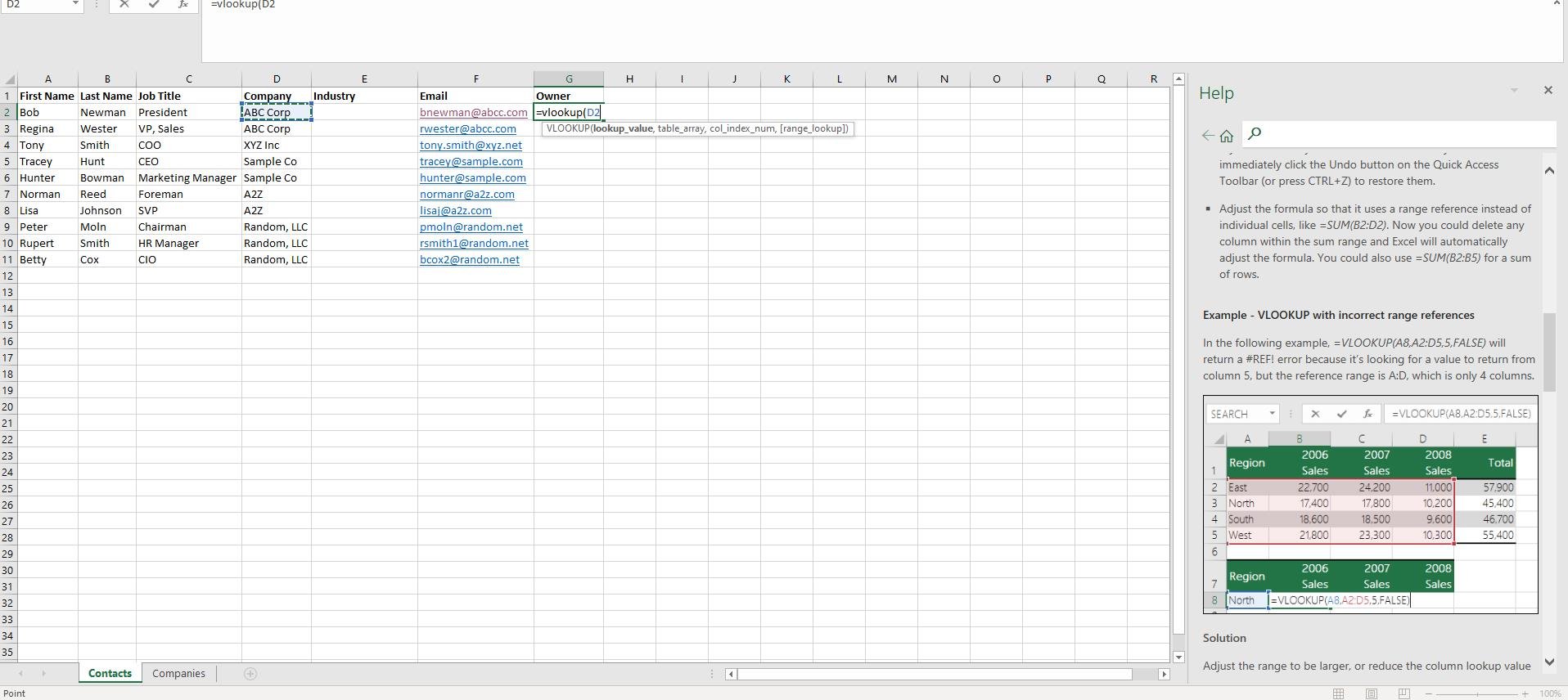
- Press "," (comma)
- Click on the tab Companies.
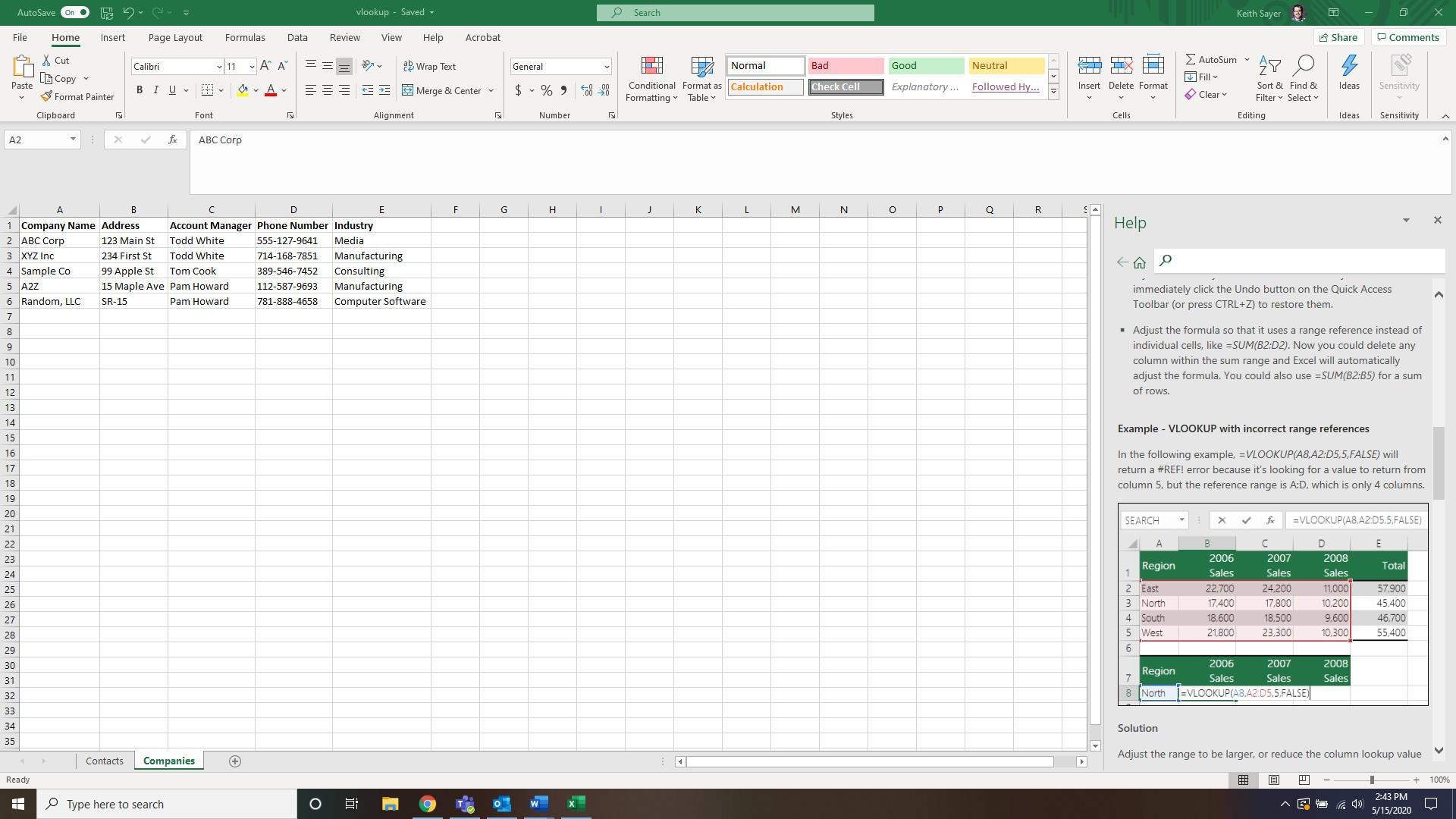
- Click and hold the left mouse button on the column header A
- Release the left mouse button on the column header E. By selecting these columns, we have effectively selected all the data in this table. Note that it is very important that the value you are looking up (in this case the Company Name) be to the left of the item you want to return (in this case, the Account Manager).
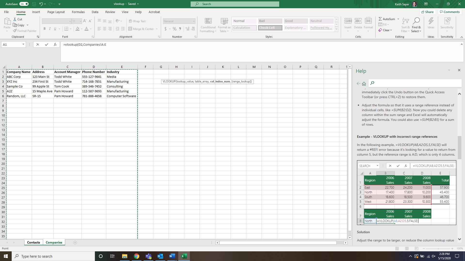
- Enter the text ,3,false). Press Enter and you will be taken back to the Contacts sheet. (3 refers to the column number of the data you want to be returned. In this case, we want the Account Manager, which is in the 3rd column. False refers to if you will accept a partial match. In this case, we want the match to be exact, so we will type out "False.")
- Click on the right part of the cell G2 with the value Todd White

- Double click on the right part of the cell G2 with the value Todd White. This pastes the formula of our first row into all subsequent rows.
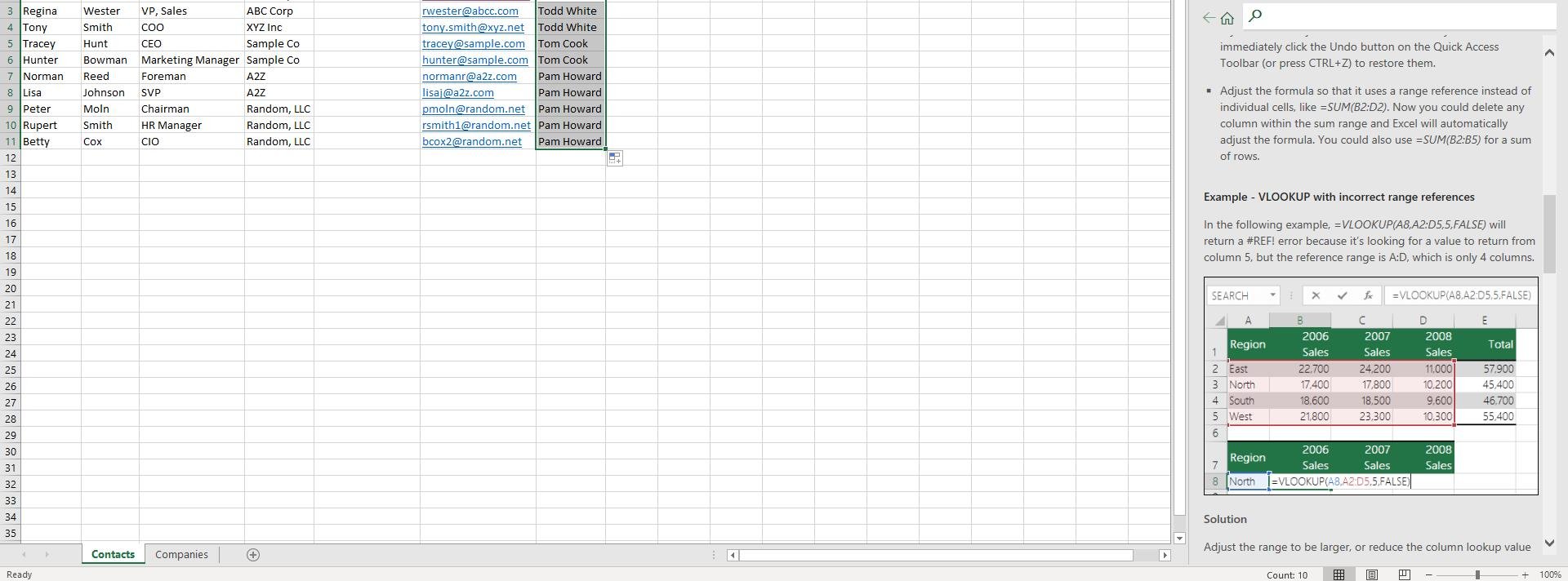
- Now let's try this on the Industry column. The process is exactly the same. Click on the cell E2.
- Enter the text =vlookup(
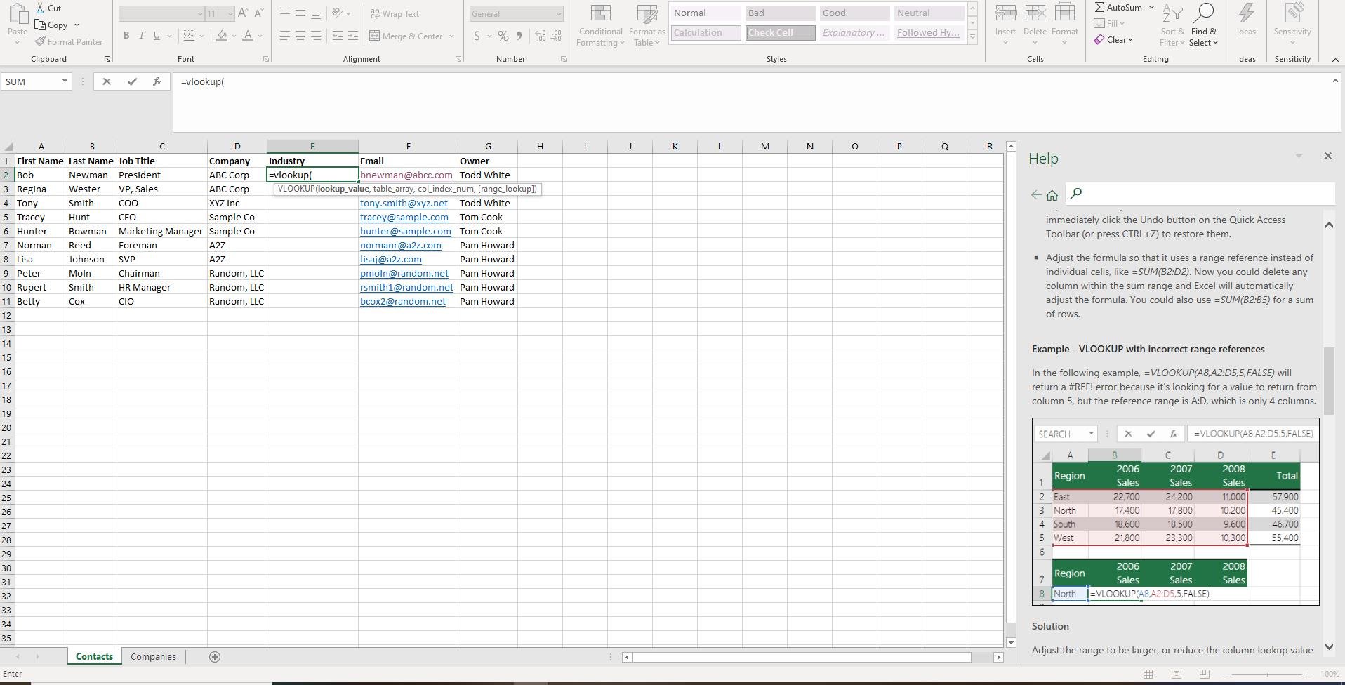
- Click on the cell D2 with the value ABC Corp
- Press "," (comma)
- Click on the tab Companies.
- Click and hold the left mouse button on the column header A
- Release the left mouse button on the column header E
- Enter the text ,5,false). Press the Enter key. (5 refers to the column number of the data you want to be returned. In this case, we want the industry of the company to come back, which is in the 5th column. False refers to if you will accept a partial match. In this case, we want the match to be exact, so we will type out "False.")

- Click on the cell E2 with the value Media
- Double click on the right part of the cell E2 with the value Media.
You can repeat this process as many times as you like to combine spreadsheets as your business process requires.
Conclusion
I hope you are already thinking of how you can use this function to manage data more efficiently in your work. It allows you to collate different spreadsheets to find the information you need to submit reports or run other functions. For example, you could take an export of data from Business Central or NAV and combine it with a spreadsheet from another program you use. Then use VLOOKUPs to make the connections.
VLOOKUP is only one of the many powerful data management tools available to you in Microsoft Excel. To learn more about what you can do with this product, consider checking out all of the Innovia blogs on this topic. Or if you want to know how to get Excel for your business, review the Microsoft 365 packages we offer at Innovia.


